Section 3: Magnetics Surveying
Introduction
Magnetics surveys measure the magnitude and orientation of the Earth’s magnetic field.
Magnetic field at Earth’s
surface depends on field generated in Earth’s core, magnetic mineral content of
surface materials, and remnant magnetisation of surface rocks.
Magnetic susceptibility, k, is physical parameter to which magnetic surveys are
sensitive.
Applications
- Location of metal
objects: Pipes,
cables, military ordnance.
- Mapping near-surface: Archeological sites, concealed
mine shafts, igneous intrusions.
- Mineral Exploration: Identification
of metalliferous deposits, for example massive sulphides
- Geological Bedrock Mapping: Identification of
faults and geological boundaries, especially beneath sediment cover.
History of Magnetics
- 2nd Century BC: Chinese used lodestone (rock
rich in magnetite) for direction finding.
- 12th Century AD: Magnetic compass in use in
Europe.
- 1600: First scientific analysis of Earth’s magnetic
field by William Gilbert in book De Magnete.
- 1640: First use of magnetic measurements to locate
iron ore deposits in Sweden.
- 1870: Development of instrumentation for rapid, accurate
measurement of magnetic field by Thalén and Tiberg.
- 1915: Development of balance magnetometer by Adolf
Schmidt.
- WWII: Rapid development of magnetic surveying
technology for mine and submarine detection.
- 1960s: Sensitive optical absorption magnetometers
allow airborne magnetics surveying.
- 1970s: Development of magnetic gradiometers to measure
field difference between two sensors.
Example of Magnetic Force, Flux, and Field
A field exists if an object placed in that field
experiences a force.
- Iron filings spread over bar magnet or around
wire carrying electric current orient in direction of magnetic field.
- Magnetic field said to exist around bar
magnet or wire, and exerts a magnetic force
that aligns the iron filings.
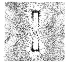
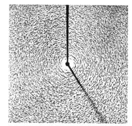
- Magnetic flux, corresponds to closeness of
field lines, and converges at magnetic poles
near ends of magnet.
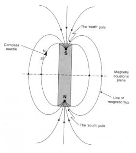
- Suspended magnet aligns itself along Earth’s
magnetic field. North-seeking (positive) pole
of magnet will point towards Earth’s north pole.
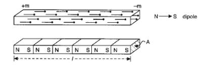
Definition of Magnetic Force
Magnetic poles always exist as dipoles,
pairs of opposite polarity, poles. If one pole sufficiently distant so does not
affect other, it is said to be a monopole.
Magnetic Force is defined in terms of monopoles:
- If two magnetic poles of strength m1
and m2 are separated by distance r, the magnitude of force
between them is given by:

where m is magnetic permeability of medium .
- Force is repulsive if poles have same sign,
attractive if opposite sign.
Magnetic Field Strength H
- Magnetic field strength vector H is
defined as force that would act on a unit positive pole placed in field:

- Magnitude of H represents "closeness"
of flux lines. Direction of H along flux lines. (assuming no
magnetic materials present).
- Magnetic field strength also defined in terms of
current flowing through a loop of wire. By Biot-Savart’s Law, the magnetic
field produced is equivalent to magnetic dipole at centre of loop.
Induced Magnetisation and Magnetic Susceptibility
Orbital motions of electrons around atoms’ nucleus
constitute circular electric currents, causing atoms to behave like magnets.
Intensity of Magnetisation J
A body placed in a magnetic field can become magnetised as
atoms and molecules align. Net external field as if bar magnet.
- Magnetic field is induced body, which is called
the intensity of magnetisation J.
(Also called magnetic polarisation).
- If J has same amplitude and direction
throughout body, body is said to be uniformly
magnetised.
Magnetic Susceptibility k
For low magnetic fields, magnetisation J is
proportional to the magnetising field H:
J = k H
where k is called the magnetic susceptibility.
- Susceptibility is fundamental rock parameter of
magnetics prospecting.
- Magnetic response of rocks determined by amounts
and susceptibilities of constituent minerals.
Total Magnetic Field B
The Total Magnetic Field B
represents the sum of the magnetising field strength and the magnetisation of
the medium:
B = m0(H + J) = m0(H + k H) = mrm0 H = m H
where m0 is magnetic permeability of free space (4p x10-7 H/m)
mr is
relative magnetic permeability
m
is absolute magnetic permeability
Clearly, mr = m / m0
B
is also called the magnetic flux density
or magnetic induction.
- Magnitude of B represents
"closeness" of flux lines. Direction of B along flux
lines.
- Magnetic field measured in volt. s /m2
= weber/m2 = teslas (T) in SI units.
- m measured in weber/ (amp.m) = henry/m (H/m)
- In c.g.s system, magnetic flux measured in gauss
or gamma 1 g = 10-5 gauss = 1
nT.
- In geophysics, magnetic fields are small and
measured in nT. Earth’s magnetic field varies between 20,000 to 60,000 nT.
B vs H
There is often confusion between B and H. In
practice, this mostly doesn’t matter, because for measurements in air mr = 1 (i.e. k = 0, can’t magnetise
air or a vacuum), and B = m0 H.
Induced and Remnant Magnetisation
Induced Magnetisation
Induced Magnetisation Ji is produced
within a rock in response to an applied external magnetic field.
Remnant Magnetisation
Magnetic field may exist within rock even in absence of
external field due to permanently magnetic particles. This is remnant or permanent
magnetisation.
Interpretation of magnetic data complicated as magnetic
field due to a subsurface body results from combined effect of two vector
magnetisations that may have different magnitudes and directions.

Diamagnetism and Paramagnetism
All atoms have a magnetic moment due to orbit of electrons
around nucleus and spin of elections moment (i.e. behave like a small bar
magnet).
According to quantum theory, two electrons can exist in same
electron shell if they have opposite spins. Magnetic moment of paired electrons
will cancel out
In most materials, no overall magnetisation exists in
absence of external field, because the magnetic moments of adjacent atoms are
randomly distributed and cancel.
Diamagnetism
- In a diamagnetic material such as halite, all electron shells are complete and
no unpaired electrons exist.
- In an external magnetic field, electrons orbit
to produce a weak magnetic field that opposes applied field.
- Magnetic susceptibility is weak and negative.
Paramagnetism
- In minerals such as olivine,
unpaired electrons in incomplete electron shells produce unbalanced
magnetic moments.
- In an external field, magnetic moments align
themselves in same direction, producing a weak magnetic field aligned with
external.
- Magnetic susceptibility is weak and positive,
but usually an order of magnitude stronger than in diamagnetic materials.
Ferromagnetism
In metals such as cobalt, nickel
and iron, unpaired electrons are coupled magnetically due to strong
interaction between adjacent atoms and overlap of electron orbits.
- Groups of atoms that couple together
magnetically are called magnetic domains,
around 1 micron in size.
- Magnetic domains can be oriented to produce a spontaneous magnetic field in absence of
external field.
- Magnetic susceptibility is large, but depends on
temperature and strength of applied field. All domains oriented in same
direction.

- Ferromagnetism disappears if material heated to Curie Temperature, TC, as
inter-atomic couping restricted and domains cannot exist.
- Behaves as paramagnetic above Cure temperature.
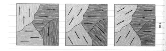
Magnetic Domains
Unmagnetised Domains
- Each domain possesses a random
magnetic field orientation.

Induced Non-Permanent Ferromagnetism
- Domains aligned with external
field grow at expense of others as external magnetic field increases.
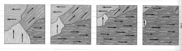
Induced Permanent Ferromagnetism
- Electrons in domains rotate to
align with external field as it increases.
Antiferromagnetism and Ferrimagnetism
Antiferromagnetism
- In minerals such as hematite,
magnetic domains form, but are aligned in antiparallel fashion.
- Magnetic fields cancel out, but crystal lattice
defects cause small net field in response to applied external field.
- Magnetic susceptibilities are large and
positive.
Ferrimagnetism
- In minerals such as magnetite,
titanomagnetite, and ilmenite,
magnetic domains are antiparallel, but of unequal magnitude.

- Net magnetisation produced with applied external
field.
- Magnetic susceptibilities are very large and
positive.
- Domains can be permanently aligned, producing
spontaneous magnetisation that exists after removal of external field.
- Ferrimagnetism disappears above Cure
temperature.
Magnetisation of Ferromagnetic Materials
Magnetisation
- For an unmagnetised material with magnetic
domains in absence of external magnetic field H, domain orientation
related to crystal axes and magnetisation cancels out.
- When external field H is applied, domains
reorient themselves in discrete steps to parallel H.
- Point is reached where no further increase in
magnetisation, as all domains aligned with external field H.
Material is saturated.

Hysteresis Loop in Magnetisation
- After magnetisation, ferro/ferri-magnetic
material retains magnetisation when H decreased to zero,
- Remnant magnetisation can be removed by external
reversing magnetic field.
- Magnitude of reversed magnetic field HC
, the coercivity, needed to
eliminate remnant magnetisation is measure of its "hardness" or
permanence.
- Same process can be applied in reverse to return
to full positive magnetisation. This process is called a hysteresis loop.
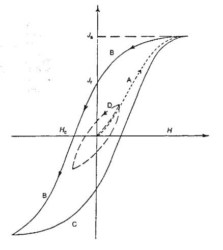
Note: Small loop is hysteresis without saturation.
Curie Temperature
Cure temperature is temperature at which mineral loses its
ferromagnetic behaviour, and any permanent magnetisation is lost.
- Cure temperature varies with mineral:
Titanomagnetite 100-200o C
Titanomaghemite 150-450o C
Magnetite 550-580o C
Hematite 650-680o C
- Curie temperature is below
melting point of rock.
- In rock such as granite, there will be multiple
Curie temperatures for the different minerals present.
Low-Temperature Oxidation
- Oxidation at less than 300o C, tends
to increase Curie temperature, as titanomagnetite oxidese towards
hematite.
- Intensity of magnetisation also reduced.
- Oxidation can affect expected magnetic response
of certain rocks.
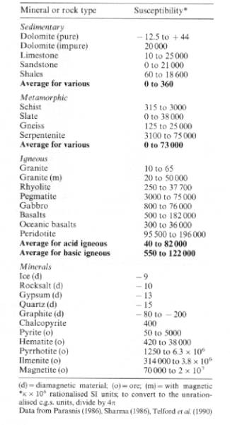
Magnetic Susceptibilities of Rocks and Minerals
Magnetic susceptibility k is the physical parameter of
magnetics surveying (equivalent to density in gravity).
Rocks with significant concentrations of
ferri/ferro-magnetic minerals have highest susceptibilities:
Ultramafic rocks highest 95,000 – 200,000
Mafic rocks high 550 – 122,000
Felsic rocks low 40-52,000
Metamorphic low 0-73,000
Sedimentary very low 0-360

Measured Values of Magnetic Susceptibility
Primary Remnant Magnetisation
Rocks can become permanently magnetised in the Earth’s
magnetic field,.
It is this that permits tracing past plate motions and
locating magnetic ores.
Primary remnant magnetisation refers to permanent magnetisation
created during formation of a rock.
Thermal Remnant Magnetisation (TRM)
- TRM acquired when a rock cools through the Curie
temperature, e.g. colling of volcanic rock.
- At Curie temperature, ferro/ferri-magnetic
minerals become magnetised in direction of Earth’s magnetic field at
that time.
- TRM usually greater than induced magnetisation
from present day field.
Detrital Remnant Magnetisation (DRM)
- DRM acquired when fine magnetic particles settle
during formation of sedimentary rock, e.g. formation of clays
- Settling particles are oriented by Earth’s
magnetic field at that time.
- DRM << TRM
Secondary Remnant Magnetisation
Secondary remnant magnetisation refers to magnetisation acquired
later in a rock’s history by alteration processes.
Chemical Remnant Magnetisation (CRM)
- CRM acquired in situ when magnetic minerals grow
or are chemically altered to another form below Curie temperature, e.g.
growth of iron oxide in sandstone.
- Most common in sedimentary and metamorphic
rocks.
Viscous Remnant Magnetisation (VRM)
- VRM produced by long exposure to ambient field
in uniform environment.
- Buildup of VRM logarithmic with time.
Königsberger Ratio
Remnant magnetisation may be much greater than that induced
by Earth’s field today, e.g. with TRM.
Königsberger Ratio Q is measure of ratio of intensity of
remnant to induced magnetisation:

- Q ~ 30-50 for rapidly quenched volcanic rocks
- Q ~10 for volcanic rocks in general
- Q~1 for slowly crystallised igneous anmd
thermally metamorphosed continental rocks
- Q<1 in sedimentary and metamorphic rocks when
iron not present
Earth’s Distant Magnetic Field
Near the Earth’s surface: magnetic field originates largely
from currents flowing in the liquid outer core, and the magnetisation of
surface rocks.
Away from the surface: magnetic field is affected by
currents caused by the movement of charged particles associated with Van Allen
radiation belts.
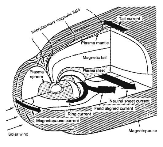
Some of these charged particles are responsible for the
Aurora Borealis near the poles.
At great distance: the magnetic field is due to charged particles from
the sun, the solar wind.
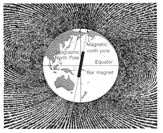
Earth’s Dipole Field
Earth’s magnetic field roughly appears as if it originated
from a large bar magnet located at the centre of the Earth oriented at 11.5o
to the axis of rotation.
Earth’s Magnetic Field
Geomagnetic Pole: the position on Earth’s surface intersected by the
axis of the dipole that fits best the Earth’s magnetic field.
o
North: Hayes
Peninsula in northern Greenland
o
South:
Vostock research station in Antarctica

Magnetic Pole (or Dip Pole): the position
where the magnetic field is vertical
o
North: North
of Bathurst Island in Canadian Arctic
o
South: 150
km offshore off Adelie coast of Antarctica
Geomagnetic and Magnetic Poles differ slightly because Earth’s magnetic field is not quite a dipole.
Generation of Earth’s Magnetic Field
Exact mechanism responsible for generation of Earth’s
magnetic field is not known.
Believed to be associated with electrical eddy currents
induced within the liquid outer core by its slow internal convection.

Secular Variation: Magnetic field is slowly changing due to core
processes, e.g. location of south magnetic pole:

Description of Earth’s Magnetic Field
A compass needle free to move in 3-D will point along the
magnetic field, i.e. it will point down where field points into Earth.
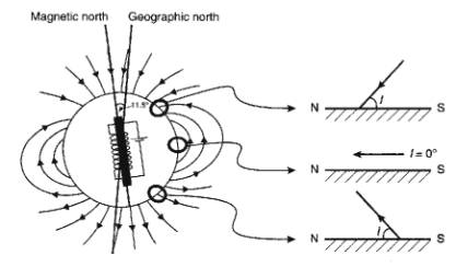
Geomagnetic field can be described by the declination D, the
inclination I, and total field vector F.

Can calculate (magnetic) latitude, l, from inclination:
![]()
Earth’s Non-Dipolar Field
90% of Earth’s magnetic field can be represented by a
dipole.
Difference between the actual magnetic field and that of the
best-fitting dipole is called the non-dipolar field.
Features in non-dipolar field with magnitudes of 20,000 nT
extending for 1000s km.
Non-dipolar field can be represented as 8-12 small dipoles
locate radially close to liquid core, simulate cores eddy currents.
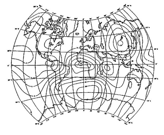
International Geomagnetic Reference Field
Geomagnetic field can be represented mathematically, and
international standard is called International
Geomagnetic Reference Field (IGRF).
Total field is recalculated every 5 years because of secular
variation. Year of calculation is called the epoch.
Total field intensity of the IGRF epoch 1980:

- A true dipole field would have two maxima, but
Earth’s magnetic field actually has four.
- IGRF excludes effects of near-surface rocks.
Variations in Earth’s Magnetic Field
Geomagnetic Reversals
Earth’s magnetic field flips polarity unpredictably on
geological time scale due to sudden changes in fluid motions in core.
Secular Variations
- Observations of Earth’s magnetic field made over
400 years show a gradual change in position of the magnetic pole.

- Due to slow movement of eddy currents in Earth’s
core.
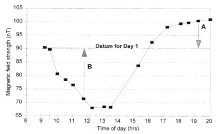
Diurnal Variations
- Daily changes in field due to changes in
currents of charged particles in ionosphere.
- Changes are smooth and average around 50 nT.
Magnetic Storms
- Short term disturbances in magnetic field
associated with sun spot activity and streams of charged particles from
sun.
- Can be up to 1000 nT in magnitude, and make
magnetic surveying impossible.
Torsion and Balance Magnetometers (Obsolete)
Magnetometers measure the total
magnetic field FT or the horizontal
and/or vertical components of magnetic field,
FH and FZ respectively.
First magnetometers devised in1640 essentially comprised:
- a magnetic needle suspended on
a wire (Torsion type), or
- a magnetic needle balanced on
a pivot (Balance type)
Needle oriented in direction of magnetic field at station
location.
Adolf Schmidt Variometer
Magnetic beam asymmetrically balanced on agate knife edge,
and zeroed at base station.
- Different magnetic field at another station
caused displacement of beam, which was measured using collimating
telescope.

- Had to be oriented perpendicular to magnetic
meridien to remove horizontal component of Earth’s field. (Use compass?)
- Calibrated to read vertical magnetic field
component.
Fluxgate Magnetometer
Measures component of magnetic field parallel to cores with
accuracy of 1-10 nT.
Comprises two parallel cores of high m ferromagnetic material.
Primary coil wound on two cores in series in opposite
directions. Secondary coils also wound, but in opposite direction to primary.

Operation of Fluxgate Magnetometer
- An alternating current at 50-1000 Hz is passed
through primary coils, producing magnetic field that drives each core to
saturation through a magnetisation hysteresis loop.
- With no external magnetic field, cores saturate
every half cycle.
- Voltages induced in secondary coils have
opposite polarity as coils wound in opposite directions. So zero net
voltage.
- In Earth's magnetic field, component of field
parallel to cores causes one core to saturate before the other, and
voltages in secondary coils do not cancel.
Principle of Operation of Fluxgate Magnetometer
- Principle behind operation is Faraday’s Law of Induction (twice)
- Voltage induced in secondary
coil proportional to magnetic field generated in ferromagnetic core.
- When core saturated, magnetic field does not
change, and no voltage is induced in secondary coil.

Proton Precession Magnetometer
Uses sensor consisting of bottle of proton-rich liquid,
usually water or kerosene, wrapped with wire coil.
Two sensors indicates a
gradiometer
- Protons have a net magnetic moment, and so are
oriented by Earth’s magnetic field or an applied field.
- Measures precession as protons reorient to
Earth’s field.
- Precession frequency proportional to total field
strength.
- As sensor bottle 15 cm long, accuracy of
measurement is reduced in areas of high magnetic field gradient.
- Measures total field strength, so instrument
orientation not important, unlike fluxgate.
- Overhauser Effect adds electron-rich fluid to
enhance polarisation effect, and increase accuracy.
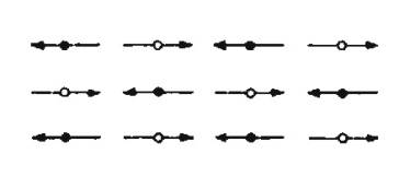
Principle of Operation of Proton Magnetometer
A.
In
ambient field, majority of protons aligned parallel to field, remainder
antiparallel.

B) Current
in coil generates strong magnetic field at right angles to Earth’s field,
causing all protons to align.
C.When current turned off protons
precess back to orientation of Earth’s field.
- Protons are charged particles, and create
magnetic field, which alternates as proton precesses.
- Current induces alternating voltage in coil at
precession frequency.
C.Measuring frequency of current in
coil gives magnitude of Earth’s total magnetic field as it is proportional to
precession frequency.
D.Measuring current frequency to 0.004
Hz gives field to ±0.1nT.
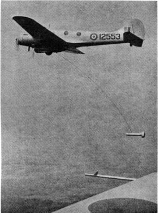
Airborne and Seaborne Magnetometers
Proton precession magnetometers are used extensively in
marine and airborne surveys:
- At sea: sensor bottle is towed in a
"fish" 2-3 ship’s length astern to remove it from magnetic field
of ship
- In air: sensor is towed 30 m behind aircraft or placed
in a "stinger" on nose, tail or wingtip.
Often active compensation for magnetic effect of aircraft is
calculated. Effectiveness of compensation is called
Figure of Merit (FOM).
Advantage:
Aeromag is rapid, cost-effective method for covering large
areas.
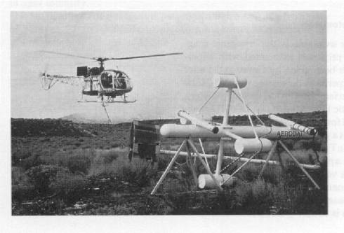
Magnetic Gradiometers
Gradiometers use two sensors separated by fixed distance to
measure gradient of the Earth’s magnetic field:
- In airborne work, separation is 2-5 m for
stinger, up to 30 m for bird.
- In ground work, separations of 0.5 m are
common.
Example of 3-axis gradiometer system:
Advantages:
- No correction for diurnal variation required as
measurement is difference off two magnetic sensors.
- Vertical gradient measurements emphasise shallow
anomalies and suppress long wavelength features.
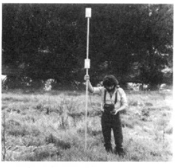
Magnetic Surveying
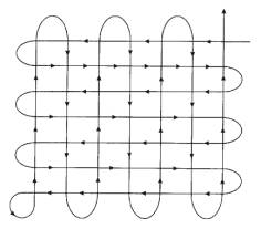
Ground Surveys
- Ideally lines should be perpendicular to strike,
with a few along strike tie-lines.
- Establish base-station to monitor diurnal
variations every 0.5-1.0 hours.
- Avoid readings near metal objects such as
railway tracks, cars...
- Avoid wearing metal objects, such as watch,
geological hammer.
Airborne Surveys
- Estimate line spacing to avoid significant
signal aliasing for aircraft height.
- Approximate rule of thumb for maximum line
spacing for particular application:

Note
that h is flight height above magnetic basement, not Earth’s surface.
Reduction of Magnetic Survey Data 1
Magnetics data reduction is usually simpler than with
gravity, comprising:
1.
Diurnal
Correction
2.
Geomagnetic
Correction
3.
Elevation/Terrain
Correction (occasionally)
Diurnal Variation
- Similar to tidal correction in gravity
- Reading is recorded at base station during
survey, and then corrections applied to survey data.
- Difficult to return to base station in airborne
work: possible to estimate diurnal correction from line intersections
especially with additional tie lines
Reduction of Magnetic Survey Data 2
Geomagnetic Correction
Similar to latitude correction in gravity: produces "anomaly" data
Earth’s total magnetic field varies from 25,000 nT at
equator to 69,000 nT at poles
Three possible correction methods:
1) Subtraction of IGRF: Earth’s theoretical magnetic
field is removed from survey data by subtracting IGRF
2) Linear approximation to IGRF: Earth’s field is
approximated by linear variation across survey area, and subtracted:
For
example, in UK IGRF is approximated by 2.13 nT/km north, and 0.26 nT/km west.
3.
Regional correction: With large surveys, regional trend can be estimated and removed to
leave residual anomaly, as with gravity data.
Terrain Correction
- There are no elevation corrections (equivalent
to Free-air and Bouguer corrections) with magnetic data as gradient is
only 0.035 nT/m at poles, 0.015 nT/m at equator.
- Terrain corrections can be applied, but are
complicated. Require estimate of ground susceptibility, and topography.

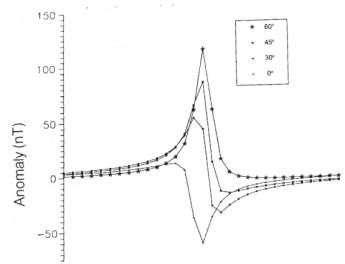
Shape of Magnetic Anomalies
Interpretation more complicated than gravity data because:
1.
Earth’s magnetic field is dipolar: single body can appear as peak and trough
Example
Vertical
component of magnetic field induced in body inclined at 60o parallel
to Earth’s magnetic field (no remnant magnetisation)
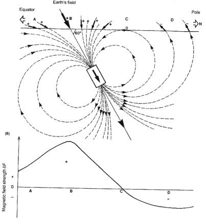
- Earth’s field removed by IGRF correction.
- Induced field strength maximum in direction of
Earth’s field.
- Sign convention: downwards is positive, negative
upwards.
- Body has negative anomaly on side towards pole
1.
Remnant magentisation unknown: strength and direction Jr can distort
anomaly shape
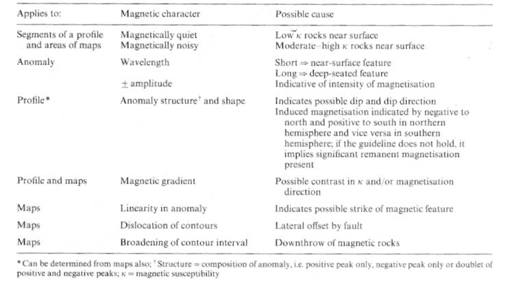
Qualitative Interpretation of Magnetic Anomalies
General inferences can be made from magnetic anomaly shapes
Example
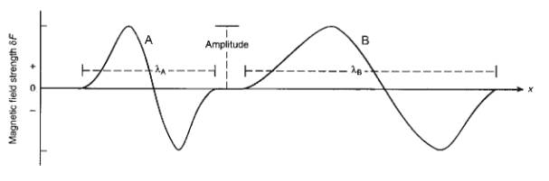
- Anomaly B is same form as A, but has longer
wavelength, so must be deeper.
- Amplitude of B greater than A, so B has greater
magnetisation.
Summary
Qualitative Profile Interpretation
Identify zones with different magnetic properties:
- Zones with little variation, "magetically quiet", associated with
rocks of low susceptibility
- Sources in subsurface in "magnetically noisy" areas.
Example: Mineralisation in granite (Dartmoor, UK)

- Profile quiet except around mineralised zone.
- Negative on north side indicates direction Ji
>>Jr as anomaly not distorted
Example: Geochemically identical dolerite dykes
(Arran, Scotland)
- Jr high as no dipolar anomaly
shape
- Two peaks and trough, intruded after magnetic
reversal
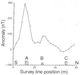
Qualitative Map Interpretation
Magnetic data acquired on ugrids can be displayed as maps
Example: Shetland Islands, Scotland

Interpretation in terms of magnetic
characteristics:
- Elongate lows correspond to gneissified
semipelites
- Can also identify fault at discontinuity
Magnetic Profile Across Buried Sphere
Magnetic data are often interpreted in terms of specific
geometric forms that approximate subsurface bodies.
Sphere or dipping sheet most common and no remnance assumed
Sphere
Example with F = 50000 nT, I=60o, D=0o,
k=0.05 for sphere radius 1 m at 3 m
depth located at x=15 m.

- Vertical and Horizontal components also shown in
addition to total field
Magnetic Profile Across Vertical Dyke
Example
Total field over 50 m thick vertical dyke with F = 50000 nT,
I=60o, D=0o, k=0.05

- Typical peak-trough anomaly arises when dyke
strikes E-W
- Anomaly is symmetric when strike is N-S. True
for all regular bodies.
Magnetic Profile Across Flat Slab
Example
Total field over 70 m thick, 400 m long flat slab located 30
m below surface with F = 50000 nT, I=60o, D=0o, k=0.05

- Slab striking N-S has symmetric anomaly
- Anomaly is broader than for thinner vertical
dyke
Effect of Change of Position on Magnetic Profile
- Change in Depth: Anomaly will broaden and
decrease in amplitude with increas in depth.
Total field over 10 m wide vertical dyke
oriented E-W

- Change in Dip: Shape of anomaly is altered
Total field over 5 m wide dyke with varying dips

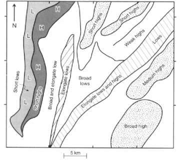
Effect of Change of Latitude
Unlike gravity, magnetic anomaly shape changes with
latitude, because orientation and magnitude of Earth’s total field varies.
Changes induced
magnetisation.
Example
5 m thick dyke dipping at 45 degrees to north with E-W
strike with different magnetic inclinations
In Northern Hemisphere:
In Southern Hemisphere:

Depth Determination
Can get very approximate depth from magnetic anomalies
Sphere or half-cylinder: Depth to centre of body w is roughly equal to width of anomaly peak at half
its maximum value dFmax/2.
Dipping Sheet or Prism: Depth to centre of body is roughly
width of linear segment of anomaly d.

Peter’s Half-Slope Method (~theoretically-based)
- Draw tangent at point of maximum slope (line 1)
- Find two tangents to curve with half maximum
slope (lines 3, 4)
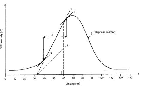
- Depth to top of body is distance between tangent
points
Application to Mineral Exploration
Example from Saramäki deposit, Finland
Target is massive copper in mineralised black schists,
beneath 30 m glacial overburden.
- Resistivity anomalies due to
black (carbon-rich) schists, not Cu
- Entire skarn zone has high density,
not just Cu, so connot see subunits


- Shows up well in magnetics
Modelling of Saramäki ore body
- Drill information suggested that magnetisation
of body heterogeneous, and upper part dominated anomaly.
- 2-D magnetics modelling could reproduce anomaly
across body, but with incorrect dip if no remanence assumed

- Including remanence with 45o
inclination and 90o declination in model allowed same match,
but with correct dip.
Detection of Underground Iron Pipes
Possible to identify underground pipes, and sometimes joints
between sections, reducing excavation required for repairs.
Each individually cast segment behaves as dipole, causing
repetition of anomalies along length
Example 1: E-W oriented pipe composed of 6.3 m segments
with diameter 0.5 m at 0.5 m depth
Gradiometer Data contoured at 200 nT/m
- Magnetic highs offset 0.5-1.0 m from joints
along pipe
- Get typical peak-trough anomaly for E-Q oriented
feature
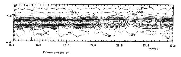
Example 2: N-S oriented pipe with 7.6 cm diameter
Gradiometer data contoured at 50 nT/m

- More symmetric anomaly due to N-S orientation of
pipe
Stanford Environmental Test Site Layout
Number of objects typical found in near surface buried in
test site, which was surveyed

Magnetics Survey of Stanford Test Site
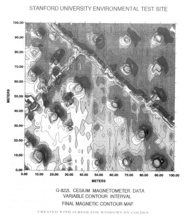
- Pipes stand out clearly due to linear trend
- Non-magnetic objects such as plastic drums or
tree stumps have minimal anomaly